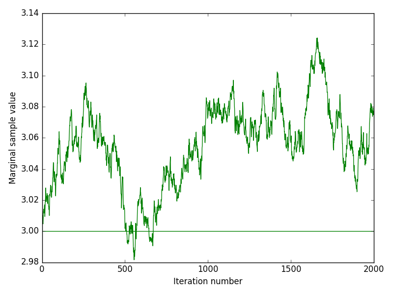
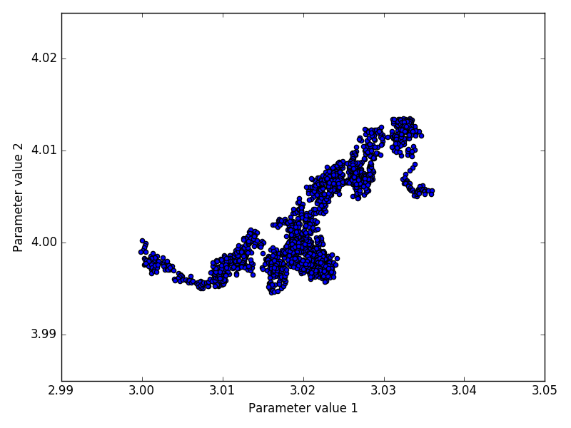
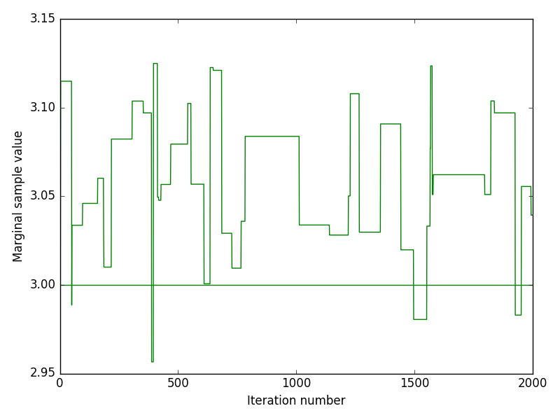
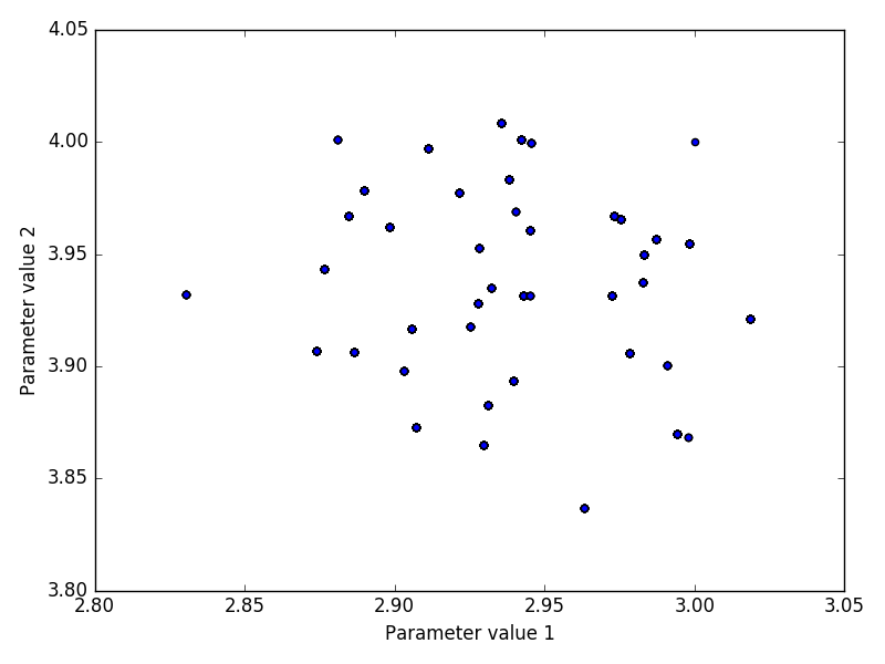
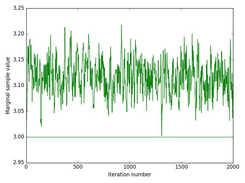
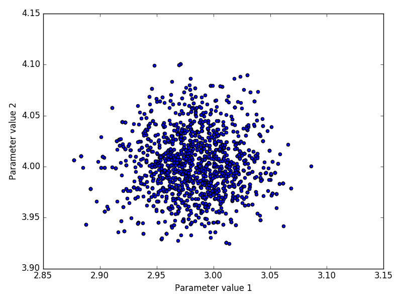
The inference method was performed on both experimental and in-silico simulated data. Below we discuss the performance of the inference by looking at indicative plots such as joint and marginal posteriors, trace plots or Bayesian credible intervals.

In-silico simulation data

We perform in-silico simulations to obtain an amplification curve given a parametrisation θ = [X₀, r, σ], a known fluorescence coefficient α (which is not inferred) and a number of qPCR cycles n. The simulated process starts with X=X₀ molecules, and is updated by sampling from a Binomial distribution with probability r. The fluorescence reads F_1:n are generated by adding noise sampled from a Gaussian distribution with variance σ (see Model).

The advantage of the in-silico data is that it allows us to compare the means and posterior distributions of all parameters X₀, r, σ with the true values using simulated data F_1:n.

In the first instance, inference was performed on data from a single amplification curve. As discussed in Inference, the exponential phase is extracted from the amplification curve and only those fluorescence reads are used as observation data. For the first ~30 cycles, the background noise dominates over the fluorescence signal, which leaves only data from ~4-5 cycles being informative for the inference of X₀ and r, before significant saturation occurs and the assumption of r being a fixed parameter is clearly unreasonable.

We found that this lack of information caused degeneracy in the inference of X₀ and r by inspecting the joint posterior of the two parameters (see below). The explanation for this phenomenon is that for a short fluorescence curve, a similar fluorescence curve can be obtained by increasing the efficiency r and lowering the quantity of the target analyte X₀ (and vice-versa). However, with more data from the "take-off" part of the curve, there would be more information to distinguish between X₀ and r.

The solution to this problem was to perform parameter-pooling inference using the data from multiple wells, with the assumption that parameters r and σ are shared between different wells within the same experimental setting. The new parameter for inference became θ = [X₀¹, X₀², X₀³, r, σ] for joint inference on 3 wells. Using data from multiple fluorescence curves where r is constant results in a more accurate inference of r, which in turn restricts the X₀^j parameters. We see that the width of the marginals is strongly constrained through this alternative model structure.

We first look at results for the data obtained from real qPCR experiments. The goal of the inference method is to perform sampling from the joint posterior distribution P(θ | F_1:n, α). The fluorescence coefficient α relates fluorescence intensity to molecule copy number and is determined prior to the inference, using sigmoid fitting on samples where the initial copy number X₀ is known. Sigmoid fitting was used instead of inference because these samples have large X₀ values, causing the process to behave deterministically (more details in Model). The inference for P(θ | F_1:n, α) produces a sequence of samples of θ that approximates the joint distribution. From this sequence we can extract samples for each component of θ (marginals) and plot the marginalised posterior distributions.

It should be noted that posteriors shown here are merely indicative due to the analysis of chain mixing, which indicates that inference needs to be run for longer (see Analysing the Markov chain).

The marginal posterior distributions are easy to visualize and encode all of our uncertainty in the parameter given the data. For the target analyte quantity X₀ we additionally plot the estimate from the standard curve method on top of the posterior distribution. The plot in Fig. 24 shows the posterior distributions obtained from joint inference using target analytes X₀¹, X₀², X₀³ from 3 separate qPCR wells (253, 254, 255).

The plots in Fig. 25 below demonstrate the effect of additional fluorescence data on the marginal posteriors by showing in parallel the results from single-well and joint inference. It is visible how the spread of posteriors narrows with joint inference, better localising the parameter values. Additionally, the prior used for each parameter is plotted: uniform prior for X₀, Jeffreys priors for r and σ (the choice of priors discussed in Priors).

In order to evaluate the inference method, we simulate a qPCR experiment in-silico and generate fluorescence data. We do so by choosing a true parameter to be the mean θ inferred from real data. An amplification curve is generated according to the random branching process model, using this fixed θ (for more details, see Model). For brevity, we only look at results from the joint inference, as it has been shown in the previous section to remove parametric degeneracy.

Testing the inference algorithm on in-silico simulated data allows the marginal posterior to be compared against a ground truth, the true parameter θ used to simulate the data, in order to check that the inference method works.

A main advantage of the Bayesian inference approach in qPCR absolute quantitation is that it accounts for both the stochasticity of the amplification process, by modelling it as a random branching process with efficiency r, as well as for parametric uncertainty. In this section, we show how stochasticity and parametric uncertainty result in a range of plausible fluorescence reads.

The inference algorithm produces a sequence of θ samples that approximate sampling from the posterior distribution of θ. A qPCR experiment was simulated in-silico for each sample, resulting in a fluorescence read sequence. A 5%-95% confidence interval for the fluorescence reads across all simulated experiments was determined at each cycle. The plotted area (Fig. 27) shows the confidence interval for the fluorescence data (green). Additionally, the plot shows the real fluorescence data used for inference (red), as well as the mean fluorescence value at each cycle (blue).

The inter- and intra-experimental variability of the fluorescence coefficient α were discussed in the Model section and are showed again (Fig. 28). Estimates for α were obtained by fitting sigmoid curves on data from standards with known initial quantities X₀. Sigmoid fitting was used instead of inference because these standards had a large copy number X₀, causing the amplification process to behave deterministically. It has been discussed that the inter-experimental variability in α is explained by the use of different primers (experiments 3 and 4 below use the same primer and have a similar distribution). Thus the α estimate can be used for inference on a new sample, if the sample uses the same primer as the standards.

We are now interested in how different values of α from the same qPCR experimental setting influence the posterior distribution of X₀, and how the initial copy number of the standard used for sigmoid fitting may play a role in the shape of the marginal posterior.

The experiments used to estimate α have the following initial standard quantities: 3 wells with 100,000 molecules, 3 with 10,000 and 3 with 1,000. A total of 9 α estimates were obtained. The plots below (Fig. 29) show posteriors from inference runs with different α values, grouped by the initial number of molecules in the curve used to determine α. The inference results plotted in other sections of this page all use the mean value of α from estimates obtained with sigmoid-fitting.

A Metropolis-Hastings algorithm produces a Markov chain of samples with the joint posterior P(θ | F_1:n, α) as its stationary distribution. The calibration of the covariance Σ of the proposal distribution Q(θ’|θ) (see General Metropolis-Hastings) is essential for producing a chain with the desired properties. Two common ways of assessing the inference method and the covariance Σ are traceplots and auto-correlation functions (ACF). We first explain the meaning of traceplots by looking at different types of Markov chains, then show the traceplots for our inference.

Background

Three types of mixing behaviour may occur:

• Chain is too cold — occurs when the covariance is too small, causing the samples to be correlated. The samples appear like a continuous trace on the joint posterior. The traceplot has fluctuations on the macroscopic level and the ACF fails to drop to zero (Fig. 30a).
• Chain is too hot — occurs when the covariance is too large, causing bad proposals and a low acceptance rate. The samples spend a long time in the same position on the joint posterior. The trace plot has a "Manhattan skyline effect" (Fig. 30b).
• Chain is well mixed — occurs when the covariance is appropriate, causing samples to appear independent and identically distributed when plotted onto the posterior. The trace plot has the "caterpillar effect" and the ACF quickly drops to zero (Fig. 30c).

Mixing results

The chains for parameters X₀ and r look cold on the macroscopic level (Fig. 31), indicating that the inference may be exploring different regions of the parameter space that are comparable in terms of their log posterior value. Inference was run for only 100,000 iterations, with equally spread 10,000 samples shown here. Therefore, the posteriors shown above are only indicative results. Running the simulations for longer may allow chains to fully mix, and should be done as future work.